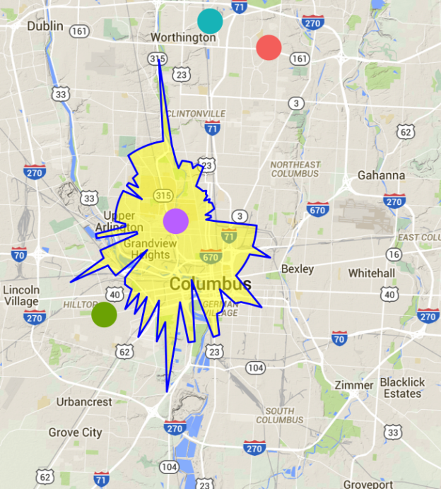
In the last post, I showed how we could use a root finding algorithm to find a drivetime isochrone around a given point. The function had two drawbacks: it evaluated the drivetime between the starting point and other locations many times, and it could only draw convex polygons. The first issue is only a problem if calling a route finder (like Google Maps) has a limit (which it typically does); the second will cause the found polygon to be slightly incorrect if the true polygon is non-convex.
Below I will show a method that finds a drivetime isochrone by evaluating the drivetime at a grid of points around the origin and then uses ggplot to draw the level curve (i.e., contour) at a given drivetime.
For this algorithm we need two R packages geosphere and ggmap.
#find a place 5 minutes away in a given direction
library(geosphere)
library(ggmap)
library(dplyr)
I will also use this crude distance function to set the bounds of the grid. This same function was defined last time.
crude_distance = function(lat,lon,distance) {
  output= data.frame(lat=distance/69,lon = 0)
  output$lon = distance/((-0.768578 - 0.00728556 *lat) * (-90. + lat))
  output
}
Finally, I will define this function that takes in the lat/lon of the origin, the desired drivetime for the isochrone, and the number of points in each direction in the grid (the total number of points the drivetime is evaluated at is this number squared). Finally, there is a multiplier that allows the user to adjust the bounds of the grid. Basically, this multiplier should be 1 if the maximum distance one can travel in one minute is 1 mile.
The function creates a grid of points around the origin and then evaluates the drive time in minutes at all these points. It returns this set of points and the drive time in minutes to get to them.
findDist <- function(lat,lon, drivetime, pts = 5, multiplier=1.0){

 #these next lines create the upper bound lat and lon using the crude_distance
 #function and then store this upper bound in a data frame
 distance = dt*multiplier
 DeltaDF = crude_distance(lat,lon,distance)
 lats <- data.frame(lat=seq(from=-DeltaDF$lat,to= DeltaDF$lat, length.out=pts) + lat)
 lons <- data.frame(lon=seq(from=-DeltaDF$lon,to= DeltaDF$lon, length.out=pts) + lon)
 distanceDF <- expand.grid(lats$lat,lons$lon)
 names(distanceDF) <- c("lat","lon")
 distanceDF <- mutate(distanceDF,loc=paste(lat,lon))
 count = 1
 for (i in 1:nrow(lats)){
   tmp <- mapdist(to=distanceDF$loc[count:(count+pts-1)], from = paste(lat,lon))
   distanceDF[count:(count+pts-1),"minutes"] = tmp$minutes
   count = count+pts
 }
 distanceDF
}
As before, remember that the Google Maps API does have limits to how many times you can call it in a given period. If you exceed that limit, the function above will give errors.
Repeating the example from the previous post gives the following result.
#get a google map for Columbus, OH
cmb = get_map("Columbus, OH", zoom= 11)

#geocode our points of interest
geocode_locations = data.frame(place=c("2762 Sullivant Ave, Columbus, OH 43204","411 Woody Hayes Dr, Columbus, OH 43210","6601 Huntley Road, Columbus, OH 43229","2300 East Dublin Granville Road, Columbus, OH"),names=c("Fine Line Ink","Ohio Stadium","Jack Maxton Chevrolet","Auto Direct Columbus"),stringsAsFactors = F)
geocode_locations[,c("lon","lat")] = geocode(geocode_locations$place)

#the desired drivetime
dt = 10

#call the function
distanceDF = findDist(lat = filter(geocode_locations, names=="Ohio Stadium")$lat, lon = filter(geocode_locations, names=="Ohio Stadium")$lon, drivetime = dt, pts=30, multiplier = 0.85 )


#format the theme for the map
theme_clean <- function(base_size = 8) {
    require(grid)
    theme_grey(base_size) %+replace%
    theme(
        axis.title      =   element_blank(),
        axis.text       =   element_blank(),
        axis.text.y = element_blank(),
        axis.text.x = element_blank(),
        panel.background    =   element_blank(),
        panel.grid      =   element_blank(),
        axis.ticks.length   =   unit(0,"cm"),
        axis.text       =  element_text(margin   =   unit(0,"cm")),
        panel.margin    =   unit(0,"lines"),
        plot.margin     =   unit(c(0,0,0,0),"lines"),
        complete = TRUE
        )
    }

#make the map
ggmap(cmb)+ stat_contour(data=distanceDF, aes(x=lon,y=lat,z=minutes),breaks=c(0,dt), geom="polygon",size=1, fill="yellow",color="blue", alpha=0.5) + geom_point(data=geocode_locations,aes(lon,lat,color=names),size=6) + scale_color_discrete("") +  theme_clean() + ggtitle(paste("Trade Area for Ohio Stadium as of", date()))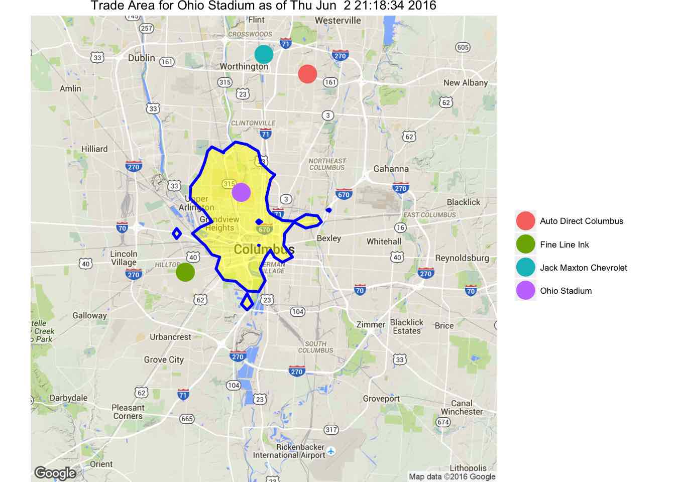
This function is a lot cleaner than the first version I posted. The results are slightly different in that the shape has changed. One interesting feature is that there are regions not connected to the main polygon. This is a result of having a finite number of points to construct the contour. Also, there is a hole in the main polygon. This means that there are points that you can’t get to in ten minutes despite the fact that there are places farther away that can be reached in ten minutes.