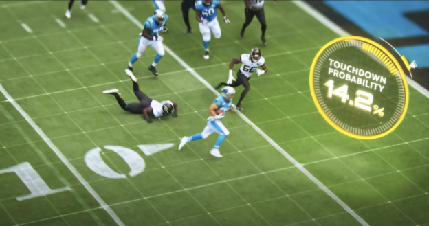
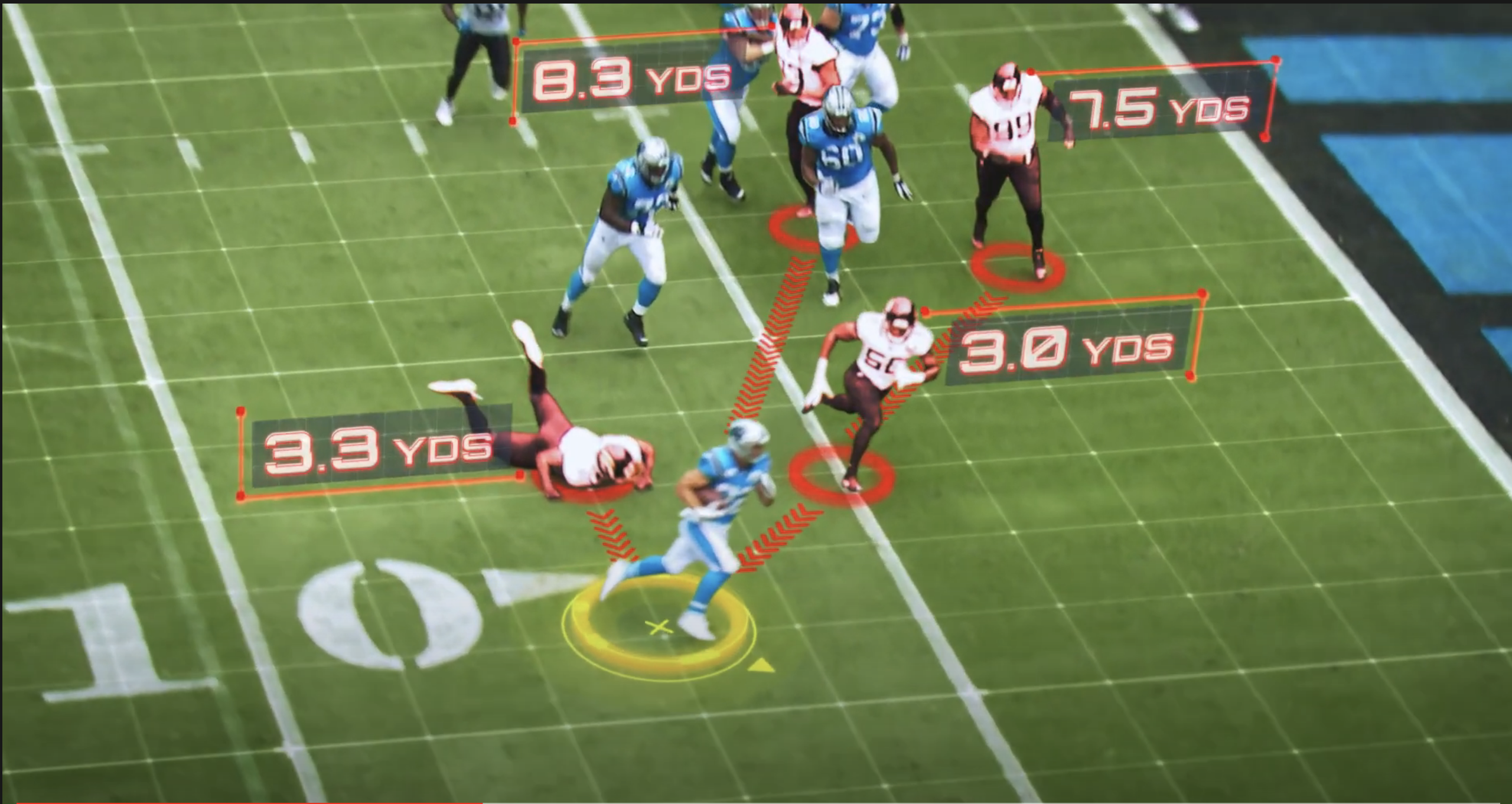
This commercial showing an exciting play where Christian McCaffery scores a touchdown has been out for some time now. In it McCaffery discusses how it was improbable (14.2% of the time or about 1/7) that a touchdown would be scored with four defenders at a given distance away (3.0, 3.3, 7.5, and 8.3 yards away). Due to the magic of “Next Gen Stats”, this play becomes a statistical anomaly. Let’s analyze this claim and see if it tells us the outcome of this play is remarkable, from a statistical point of view.
We can stipulate that for a play starting at about the 5 yard line, when there are four unblocked defenders within 8.3 yards of the runner, it is unlikely that a touchdown will be scored. I would conjecture, however, that a large majority of the time those defenders would be in front of the runner. Indeed, it might be that only 15% of the time that none of the four closest defenders are in front of the runner. In that case, the touchdown probability for the way this play initially unfolded could be 94.7% (that is, 14.2/15=0.9466…), if all of the touchdowns occurred when no defenders were in front of the runner.
An experienced football fan would look at the stills above and would bet it is more likely than not for the runner to score (even if it was clear there was a defensive back right at the goal line). This is because there is still a lot of room to the sideline and the bad angle the defender is taking. It seems like the worst possible outcome is that a tackle is made at the 2 or 3 yard line.
The fact that there are four players at the given distances does not tell us very much about the play. Indeed, it seems like two of those defenders aren’t really even running at this point. What is important, and not quantified here (possibly because it is much harder), is that none of the defenders are in the path of the runner and that the nearest defender is on the goal line.
This is an example of using the data at hand to make a decision that doesn’t really have any insight. Looking at the available data, we can infer that yes, if there are that many unblocked players, that close to a runner, it is unlikely he will score. Of course, most of those plays will be cases where the runner is swarmed in the backfield by defenders that surround him from the start of the play. However, once we have a bit more information, like that none of those defenders stand between the runner and the end zone, it becomes much more likely to score a touchdown. The eye test would tell you that the probability is much better than the roughly 1 in 7 chance this play has a score a touchdown.